Statistical Mechanics and Thermodynamics

The foundation of the GLAM framework is the adaptation of rigorous formalism from statistical physics and thermodynamics to quantify the biological organization of a tumor. By treating voxels of differing intensities as interacting particles, we can quantify the effective “interactions” shaping tumor architecture.

Radial Distribution Function (RDF)

The core descriptor is the pair radial distribution function, \(g_{\alpha\beta}(r)\), which measures the spatial correlation between voxels. It quantifies the relative likelihood of finding a voxel with gray level \(\beta\) at a distance \(r\) from a reference voxel with gray level \(\alpha\).

• Positive Correlation (Attraction): \(g_{\alpha\beta}(r) > 1\).

• Negative Correlation (Repulsion): \(g_{\alpha\beta}(r) < 1\).

• Randomness: \(g_{\alpha\beta}(r) = 1\).

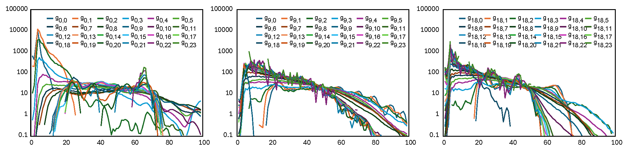
Figure: RDF as a function of the distance \(r\) (from 0 to 100 mm). Each colored line represents a specific RDF curve, \(g_{\alpha\beta}(r)\), between two different gray levels, \(\alpha\) and \(\beta\).

• Interpretation: This metric asks, “How much more or less likely am I to find tissue type B at a specific distance from tissue type A, compared to a completely random distribution?”

• Advantage: It provides a fundamental, distance-dependent map of spatial relationships rather than just a single global average, revealing exact distances where tissues cluster or repel.

RDF Shape Statistics

To capture the extensive information embedded in the full RDF curves without incurring the “curse of dimensionality,” we transform key statistical properties of each \(g_{\alpha\beta}(r)\) curve into a set of primary GLAM matrices. For every gray-level pair, we compute the Peak Position, Dispersion Ratio, Peak Height, Median, Variance, Skewness, and Kurtosis.

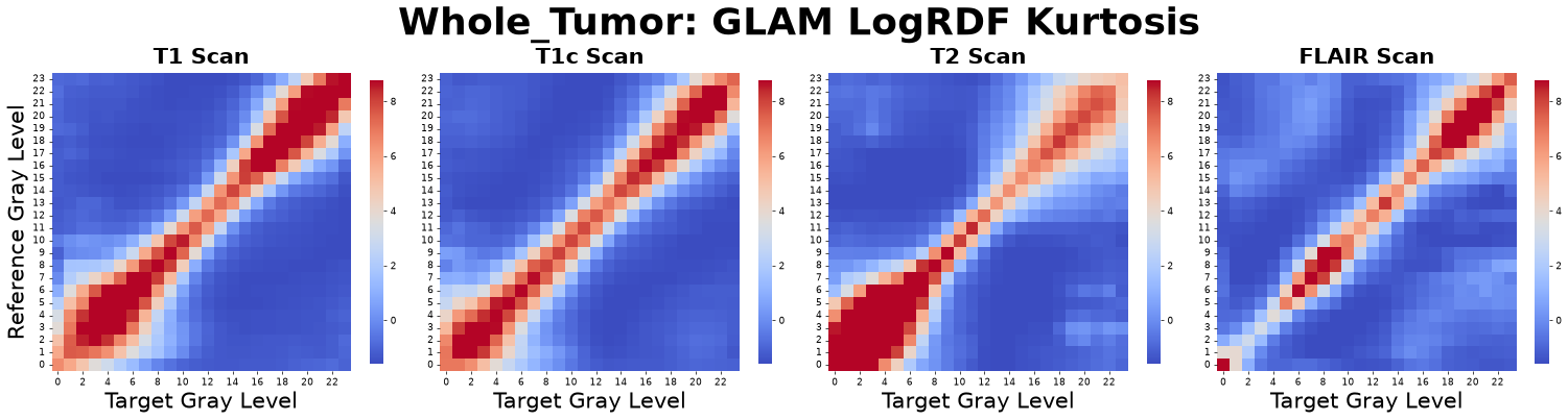
Figure: RDF Kurtosis matrices derived from four co-registered MRI sequences: pre-contrast T1-weighted (T1), post-contrast T1-weighted (T1c), T2-weighted (T2), and Fluid-Attenuated Inversion Recovery (FLAIR).

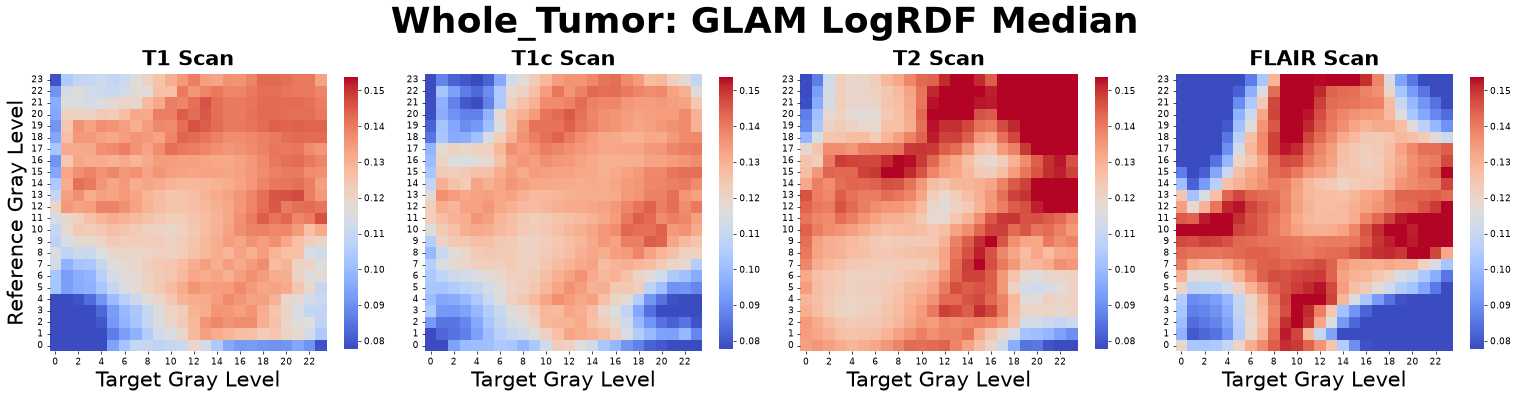
Figure: RDF Median matrices derived from four co-registered MRI sequences: pre-contrast T1-weighted (T1), post-contrast T1-weighted (T1c), T2-weighted (T2), and Fluid-Attenuated Inversion Recovery (FLAIR).

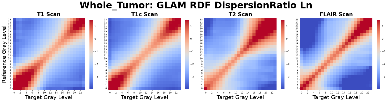
Figure: RDF Dispersion Ratio matrices derived from four co-registered MRI sequences: pre-contrast T1-weighted (T1), post-contrast T1-weighted (T1c), T2-weighted (T2), and Fluid-Attenuated Inversion Recovery (FLAIR).

Key Thermodynamic Metrics

Second Virial Coefficient (\(B_2\))

The second virial coefficient distills the complex, distance-dependent information of the entire RDF curve into a single value representing net affinity.

\[B_{2\alpha, \beta} = -2\pi \int_{0}^{R_{max}} [g_{structured}(r) - g_{randomized}(r)] r^2 dr\]

• Negative value: Indicates net attraction or affinity between gray levels.

• Positive value: Suggests net repulsion.

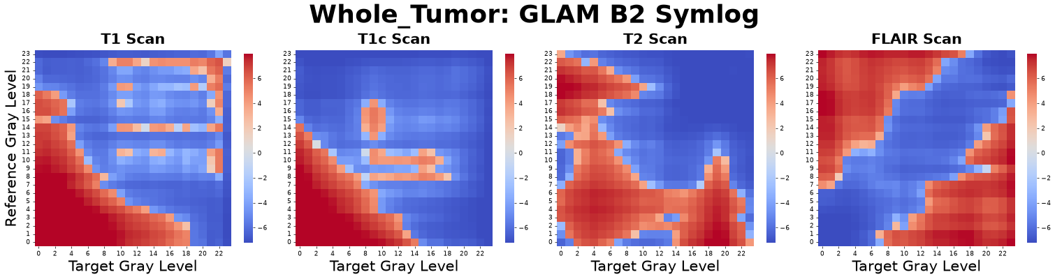
Figure: B2 matrices derived from four co-registered MRI sequences: pre-contrast T1-weighted (T1), post-contrast T1-weighted (T1c), T2-weighted (T2), and Fluid-Attenuated Inversion Recovery (FLAIR).

• Interpretation: This metric asks, “Overall, do these two tissue types prefer to clump together (attraction) or push each other apart (repulsion) across the entire tumor?”

• Advantage: It condenses a complex multi-distance curve into a single, highly interpretable summary statistic of spatial affinity.

Potential of Mean Force (PMF)

To evaluate the energetic stability of texture organization, GLAM computes the PMF based on the Boltzmann distribution.

\[W_{\alpha\beta}(r) = -k_B T \ln g_{\alpha\beta}(r)\]

The total PMF energy is obtained by integrating this potential weighted by the RDF:

\[U_{PMF\alpha,\beta} = 4\pi \int_{0}^{R_{max}} W_{\alpha\beta}(r) g_{\alpha\beta}(r) r^2 dr\]

To allow size-independent comparison across ROIs, the UPMF is normalized by volume, producing the Energy Density, which represents the average interaction energy per voxel.

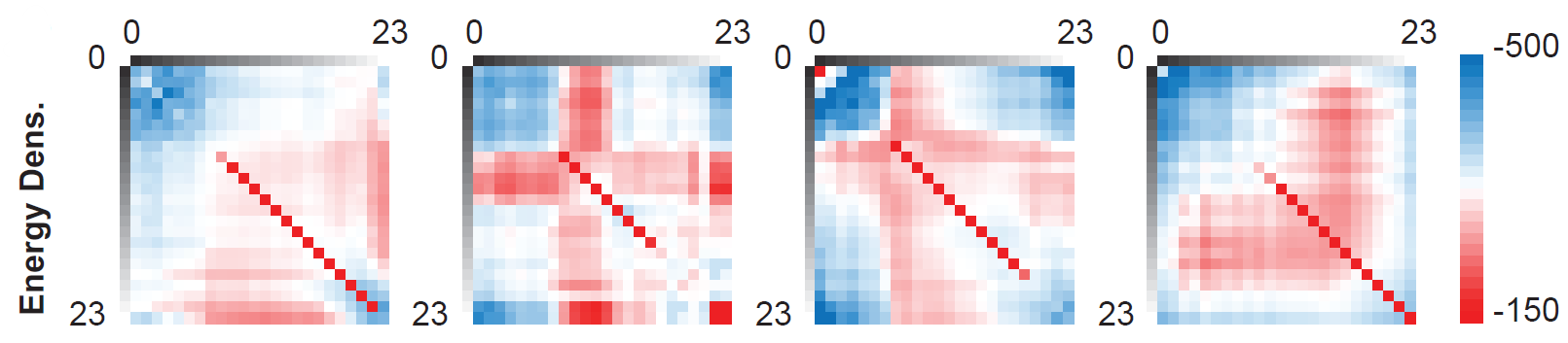
Figure: Energy Density matrices derived from four co-registered MRI sequences: pre-contrast T1-weighted (T1), post-contrast T1-weighted (T1c), T2-weighted (T2), and Fluid-Attenuated Inversion Recovery (FLAIR).

• Interpretation: This metric asks, “How much ‘energy’ would it take to maintain this specific spatial arrangement of tissues against natural thermodynamic mixing?”

• Advantage: It translates geometric clustering into a physical energy landscape, allowing the identification of highly stable (deep energy wells) versus unstable, transient tissue architectures.

Isothermal Compressibility (\(\kappa_T\))

In statistical thermodynamics, the integral of the total correlation function is directly related to the system’s density fluctuations and its isothermal compressibility.

\[\kappa_T \propto \int_{0}^{R_{max}} [g_{\alpha\beta}(r) - 1] r^2 dr\]

In the GLAM framework, this metric quantifies the “sponginess” or susceptibility of the texture to local density variations. High compressibility implies large-scale density fluctuations and a tendency for the voxel population to cluster loosely, whereas low compressibility indicates a rigid, hyper-uniform distribution typical of highly packed cellular structures.

---

• Interpretation: This metric asks, “How ‘spongy’ or susceptible to density fluctuations is the tissue architecture?”

• Advantage: It captures large-scale structural heterogeneity. Low compressibility indicates rigid, tightly packed regions (like dense stroma), while high compressibility flags loose, highly variable clustering.

Structural Pressure Index (\(SPI\))

Broadly analogous to the virial equation of state, the Structural Pressure Index (SPI) utilizes a PMF-derived potential of mean force, \(W_{\alpha\beta}(r)\), to serve as a pressure-like structural descriptor. It quantifies the mean pseudomechanical force between voxel populations, capturing the spatial packing and mechanical-like response within the texture.

\[SPI_{\alpha,\beta} = -\frac{\rho_\alpha \rho_\beta}{6} \int_{0}^{R_{max}} r \frac{dW_{\alpha\beta}(r)}{dr} g_{\alpha\beta}(r) 4\pi r^2 dr\]

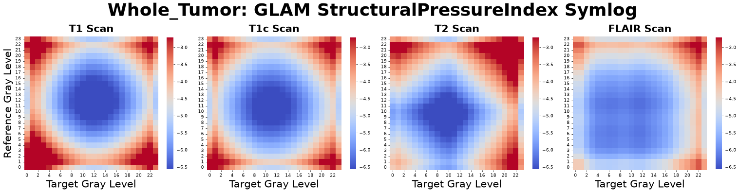
Figure: Structural Pressure Index matrices derived from four co-registered MRI sequences: pre-contrast T1-weighted (T1), post-contrast T1-weighted (T1c), T2-weighted (T2), and Fluid-Attenuated Inversion Recovery (FLAIR).

• Interpretation: This metric asks, “What is the net ‘push or pull’ (internal spatial stress) exerted between different voxel populations due to their structural arrangement?”

• Advantage: It links spatial statistics directly to thermodynamic concepts, offering a non-invasive computational proxy for the internal architectural stresses within the tumor microenvironment.

Configurational Disorder Index (\(CDI\))

To complement metrics of energetic stability, the Configurational Disorder Index (\(CDI\)) characterizes textural disorder. Whereas PMF energy assesses how stable the structure is, the \(CDI\) quantifies how dynamically disordered it is. The \(CDI\) is derived by comparing the measured RDF of the actual image, \(g_{structured}(r)\), to that of its randomized counterpart, \(g_{randomized}(r)\).

Drawing from the Boltzmann relation, which links the probability of a configuration to its energy and relative disorder, deviations from randomness reflect an underlying “ordering potential.” Because \(\ln(g(r))\) is proportional to the negative potential divided by this disorder parameter, the observed structure, \(\ln(g_{structured}(r))\), represents this potential modulated by the tissue’s inherent architectural chaos. The ratio between the structured and randomized forms yields a distance-dependent disorder profile:

\[CDI(r) = \frac{\ln(g_{structured}(r))}{\ln(g_{structured}(r)) - \ln(g_{randomized}(r))}\]

Averaging \(CDI(r)\) within the first coordination shell yields a stable, physically interpretable estimate of the local structural disorder, \(CDI(\alpha,\beta)\). A high \(CDI(\alpha,\beta)\) indicates greater structural “noise” or heterogeneity, while a low \(CDI\) indicates rigid or highly structured ordering. Comparing diagonal versus off-diagonal \(CDI(\alpha,\beta)\) elements distinguishes self-organized tissue components from dynamically disordered interfaces.

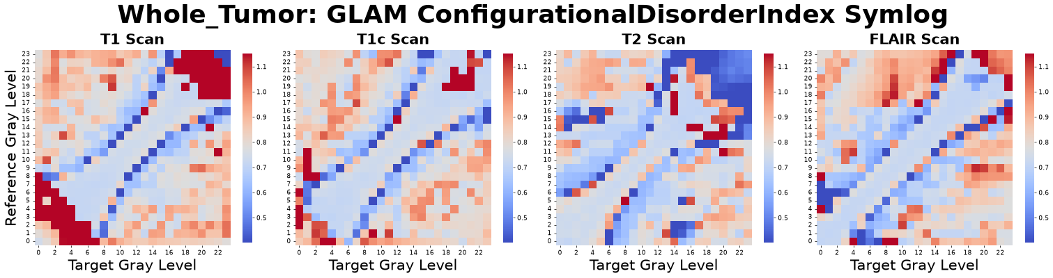
Figure: Configurational Disorder Index matrices derived from four co-registered MRI sequences: pre-contrast T1-weighted (T1), post-contrast T1-weighted (T1c), T2-weighted (T2), and Fluid-Attenuated Inversion Recovery (FLAIR).

• Interpretation: This metric asks, “How much structural ‘noise’ or configurational disorder exists in this tissue compared to a perfectly ordered state?”

• Advantage: It provides a clear indicator of architectural chaos; highly disordered tissues appear random and heterogeneous, while low-disorder tissues are rigidly structured. This thermodynamic-inspired approach provides a robust, physically interpretable measure of local architectural complexity in medical images.

1-Wasserstein Distance (Assembly Cost)

The 1-Wasserstein Distance, often called the Earth Mover’s Distance (EMD), measures the “Biological Work” or “Assembly Cost” of the tumor’s spatial architecture. It quantifies the total effort required to transform a completely randomized spatial distribution of voxels into the highly ordered, structured state actually observed in the tumor.

First, the Cumulative Coordination Number, \(N(R)\), is calculated. This represents the total number of neighbors accumulated up to radius \(R\):

\[N(R) = \int_0^R 4\pi \rho_\beta g(r) r^2 dr\]

The Wasserstein distance is then defined as the absolute area between the cumulative curves of the structured and randomized states:

\[W_{\alpha\beta} = \int_{0}^{R_{max}} \left| N_{structured}(R) - N_{random}(R) \right| dR\]

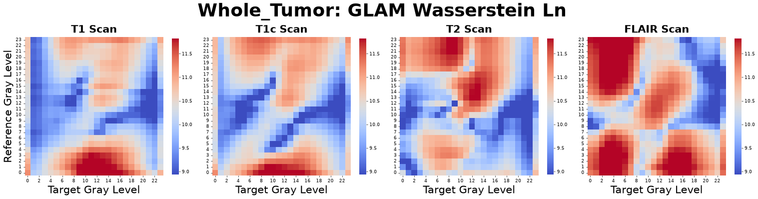
Figure: Wasserstein matrices derived from four co-registered MRI sequences: pre-contrast T1-weighted (T1), post-contrast T1-weighted (T1c), T2-weighted (T2), and Fluid-Attenuated Inversion Recovery (FLAIR).

• High Value: Indicates a highly complex, non-random architecture with a high energetic “cost” of assembly, typical of highly organized distinct sub-regions or rigid boundaries.

• Low Value: Indicates the tissue architecture is very close to a completely random distribution of cells or voxels.

Assembly Coupling Matrix (Thermodynamic Entanglement)

The Assembly Coupling Matrix measures the thermodynamic entanglement between different tissue states. By taking the mixed partial derivative of the 1-Wasserstein Distance (Assembly Cost) with respect to both the reference state \(\alpha\) and target state \(\beta\), it quantifies how the structural formation of one gray level interferes with or facilitates another.

\[\mathcal{X}_{\alpha\beta} = \frac{\partial^2 W_{\alpha\beta}}{\partial \alpha \partial \beta}\]

Because the raw derivative values scale exponentially at phase boundaries, a Symmetric Logarithm (SymLog10) transform is applied to compress extreme magnitudes while strictly preserving the thermodynamic sign.

• Positive Value (Antagonistic Assembly): The two tissue states structurally compete for the same microenvironmental space (e.g., an expanding solid core pushing against an unyielding stroma).

• Negative Value (Synergistic Assembly): The states are structurally cooperative, where the presence of one lowers the thermodynamic barrier to assemble the other (e.g., angiogenesis actively facilitating dense cellular packing).

• Zero Value: Structural independence.

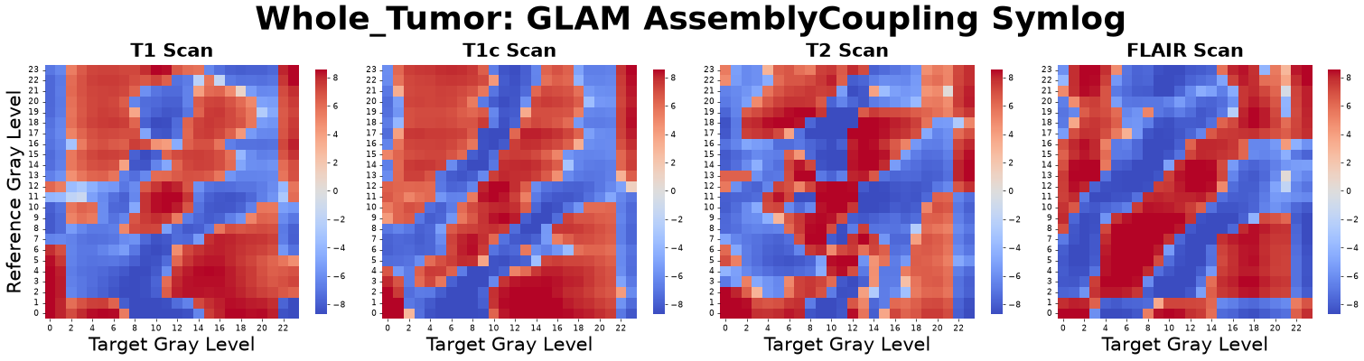
Figure: Assembly Coupling matrices derived from four co-registered MRI sequences: pre-contrast T1-weighted (T1), post-contrast T1-weighted (T1c), T2-weighted (T2), and Fluid-Attenuated Inversion Recovery (FLAIR).

• Interpretation: This metric asks, “If the tumor mutates to increase tissue type B, does that make it biologically harder (antagonistic) or easier (synergistic) to build tissue type A?”

• Advantage: It distills complex topological and thermodynamic states into a pure map of biological alliances and competitions within the tumor ecosystem.

Phenotypic Distance Matrix (Phase-Space EMD)

Instead of comparing a tissue state to a randomized baseline, the Phenotypic Distance Matrix directly compares the morphological architecture of two distinct gray levels, \(\alpha\) and \(\beta\). It computes the 1-Wasserstein Distance between their normalized auto-correlation Cumulative Distribution Functions (CDFs), \(F(r)\).

\[\mathcal{W}_{\alpha \rightarrow \beta} = \int_{0}^{R_{max}} \left\vert{} F_\alpha(r) - F_\beta(r) \right\vert{} dr\]

This produces a strictly non-negative, perfectly symmetric distance matrix (\(\mathcal{W}_{\alpha \rightarrow \beta} = \mathcal{W}_{\beta \rightarrow \alpha}\)) with zeros along the main diagonal. Because it is a true distance metric bounded by the maximum integration radius, no downstream logarithmic transformations are required.

• Low Value (Morphological Mimicry): The two states have highly similar spatial topologies, meaning the tissue can shift intensities with nearly zero topological reorganization cost.

• High Value (Structural Barrier): The states possess vastly different spatial architectures, requiring massive biological energy to physically tear down and rebuild the tissue topology during a phase transition.

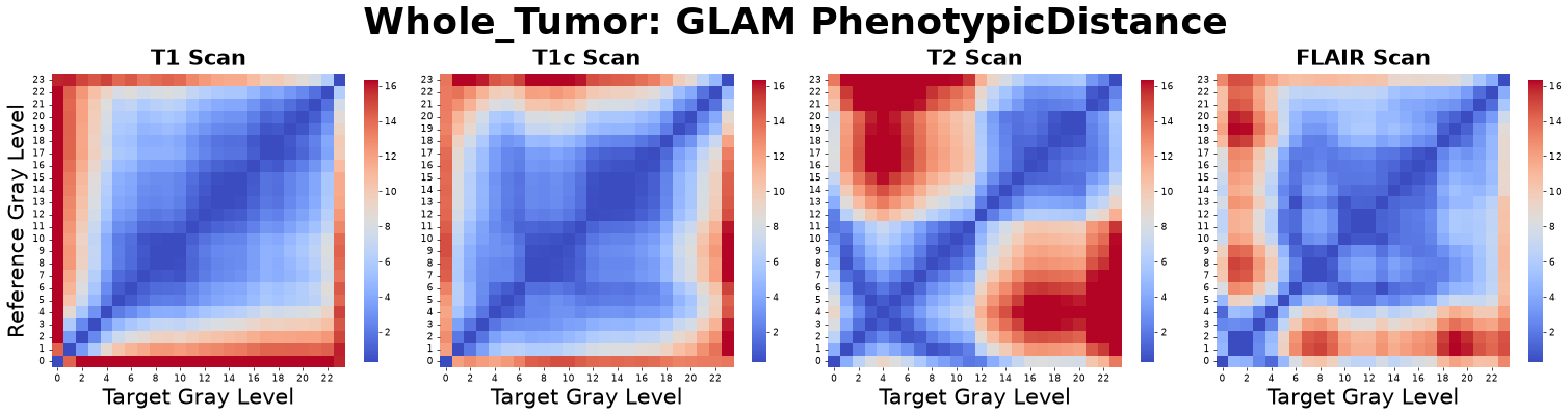
Figure: Phenotypic Distance matrices derived from four co-registered MRI sequences: pre-contrast T1-weighted (T1), post-contrast T1-weighted (T1c), T2-weighted (T2), and Fluid-Attenuated Inversion Recovery (FLAIR).

• Interpretation: This metric asks, “Regardless of their contrast intensity, how physically similar are the spatial packing architectures of tissue A and tissue B?”

• Advantage: It provides a true mathematical distance metric in morphological phase-space, allowing downstream clustering algorithms to objectively group distinct gray levels into physically identical “habitats.”

Mechanical Phase and Jamming Transitions

These metrics describe the underlying mechanical phase state of the tissue architecture, determining whether a local microenvironment behaves as a structurally arrested (solid-like) mass or a yielding, invasive (fluid-like) network.

Local Packing Fraction (\(\Phi\))

The Local Packing Fraction grounds abstract spatial relationships into a dimensionless, scale-invariant volume ratio. It measures the exact physical volume fraction occupied by neighboring gray levels within the first coordination shell, utilizing dynamic boundary-intersection normalizations.

\[\Phi_{\alpha\beta} = \frac{CN_{\alpha\beta}}{V_{shell}(r_{min})}\]

where \(CN_{\alpha\beta}\) is the Coordination Number and \(V_{shell}(r_{min})\) is the exact geometric volume of the coordination shell.

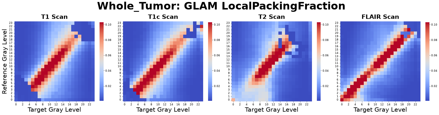
Figure: Local Packing Fraction matrices derived from four co-registered MRI sequences: pre-contrast T1-weighted (T1), post-contrast T1-weighted (T1c), T2-weighted (T2), and Fluid-Attenuated Inversion Recovery (FLAIR).

• Interpretation: This metric asks, “Exactly what percentage of the available physical space around a central voxel of type A is consumed by voxels of type B?”

• Advantage: It is inherently bounded between 0.0 (empty) and 1.0 (perfectly solid), providing a highly tangible measure of micro-regional crowding and spatial saturation without requiring downstream mathematical transformations like log scaling.

Structural Frustration Index (\(\mathcal{F}\))

The Structural Frustration Index mathematically isolates the thermodynamic conditions required for a solid-to-fluid unjamming transition. It is defined as the ratio of local structural stress to local configurational disorder:

\[\mathcal{F}_{\alpha\beta} = \frac{SPI_{\alpha\beta}}{CDI_{\alpha\beta} + \epsilon}\]

where \(SPI_{\alpha\beta}\) is the Structural Pressure Index, \(CDI_{\alpha\beta}\) is the Configurational Disorder Index, and \(\epsilon\) is a small regularization constant to prevent division by zero in highly ordered (crystalline) regions.

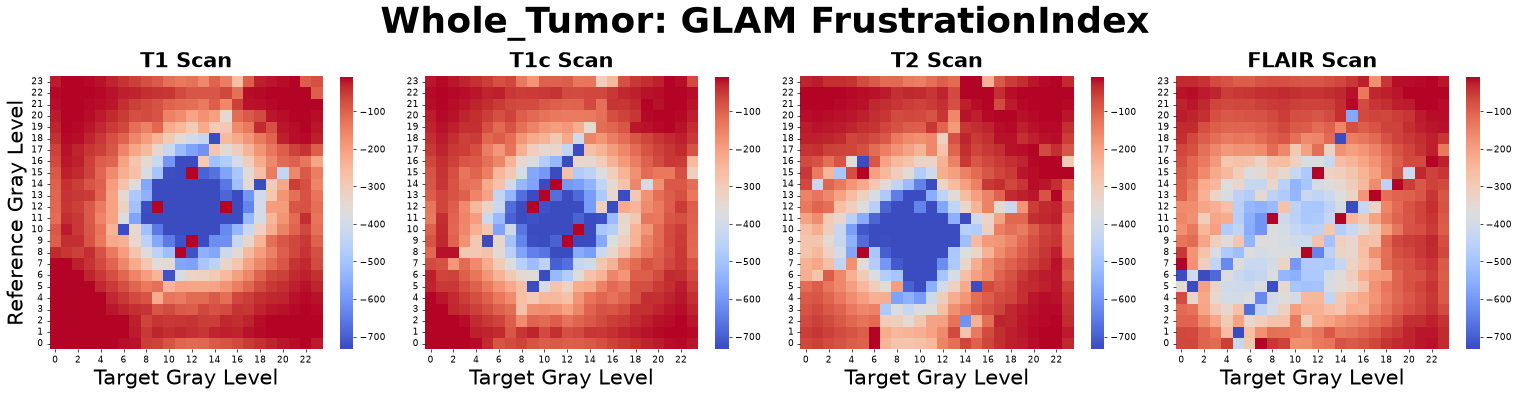
Figure: Structural Frustration Index matrices derived from four co-registered MRI sequences: pre-contrast T1-weighted (T1), post-contrast T1-weighted (T1c), T2-weighted (T2), and Fluid-Attenuated Inversion Recovery (FLAIR).

• Interpretation: This metric asks, “Is this tissue microenvironment jammed under high structural tension but unable to rearrange (high frustration), or is it yielding and fluid-like (low frustration)?”

• Advantage: By combining pressure and disorder into a single non-linear filter, it creates massive mathematical contrast between structurally locked cores and actively invading, unjammed margins. It acts as a highly sensitive macroscopic phase identifier for prognostic modeling.

Note on the Removal of JS Divergence (Asymmetry)

In earlier versions of GLAM, the Jensen-Shannon (JS) Divergence was calculated to measure the structural asymmetry between two interacting tissues by comparing the probability distribution of finding tissue B around A (g_ij) versus finding tissue A around B (g_ji).

This feature has been formally deprecated and removed from the pipeline due to the thermodynamic law of Global Reciprocity.

In statistical mechanics, the unnormalized pair correlation functions are strictly bound by the global volumetric densities (ρ) of the two tissues:

g_ij(r) * ρ_j = g_ji(r) * ρ_i

To compare these curves using Information Theory (like JS Divergence or Kullback-Leibler), they must first be L1-normalized into true probability distributions (P and Q). Because g_ij and g_ji differ only by a scalar constant, dividing them by their respective sums completely cancels out the volumetric density constant.

Mathematically, this forces the normalized distributions to be identical (P(r) == Q(r)). Therefore, the theoretical JS Divergence between any two tissues in the GLAM framework is exactly 0.0.

What this means for users: We found that any non-zero JS Divergence values produced by the pipeline were strictly the result of microscopic stochastic variance during the random sampling phase (shot noise), not true biological signal. To ensure mathematical purity and prevent “junk” features from entering downstream machine learning models, these matrices were removed.

Users wishing to measure the asymmetry and directional alignment of tumor structures should refer to the Gyration Tensor Anisotropy (GLAM_Anisotropy_matrix) and the Interface Area (GLAM_Shape_InterfaceArea_matrix) features, which perfectly capture non-reciprocal topological behaviors.

Jensen-Shannon (JS) Divergence

While the standard RDF quantifies the distance-dependent interaction between two specific gray levels, comparing reciprocal RDF curves allows us to evaluate the directional symmetry—or structural anisotropy—of this relationship. In a perfectly isotropic (directionless) texture, the probability of finding gray level \(\beta\) at distance \(r\) from gray level \(\alpha\) should be identical to finding gray level \(\alpha\) at distance \(r\) from gray level \(\beta\). Therefore,

\[g_{\alpha\beta}(r) \approx g_{\beta\alpha}(r).\]

JS Divergence quantifies the disagreement between these two reciprocal RDF curves. Because standard Kullback-Leibler (KL) Divergence is asymmetric and struggles with zeros, JS Divergence creates a symmetric, bounded comparison by measuring how far both curves deviate from their shared average.

First, the raw RDF curves are L1-normalized into true probability distributions, \(P\) and \(Q\):

\[P(r) = \frac{g_{\alpha\beta}(r)}{\sum g_{\alpha\beta}(r)}\]

\[Q(r) = \frac{g_{\beta\alpha}(r)}{\sum g_{\beta\alpha}(r)}\]

We define a midpoint distribution \(M\):

\[M(r) = \frac{1}{2} (P(r) + Q(r))\]

The JS Divergence is then calculated as the average KL Divergence of \(P\) and \(Q\) from \(M\):

\[JSD(P \parallel Q) = \frac{1}{2} \sum P(r) \log_2 \left( \frac{P(r)}{M(r)} \right) + \frac{1}{2} \sum Q(r) \log_2 \left( \frac{Q(r)}{M(r)} \right)\]

• Perfect Symmetry (\(JSD = 0\)): The relationship between tissue A and tissue B is structurally identical in reverse.

• Structural Anisotropy (\(JSD > 0\)): Tissue B tends to cluster around tissue A differently than tissue A clusters around tissue B (e.g., A forms a core while B forms a shell).

---

• Interpretation: This metric asks, “Is the local neighborhood of tissue A around tissue B an exact mirror image of tissue B around tissue A?”

• Advantage: It offers a bounded (0 to 1) and perfectly symmetric measure of local directional bias, avoiding the mathematical instabilities of traditional Kullback-Leibler divergence when encountering empty tissue regions.

Cumulative JS Divergence

Raw RDF curves (\(g(r)\)) can be noisy, especially in small tumors or sparse gray levels, causing artificial spikes in standard JS Divergence.

Cumulative JS Divergence solves this by borrowing intuition from the Wasserstein metric (Earth Mover’s Distance). Instead of comparing local densities shell-by-shell, it compares the Cumulative Coordination Profiles—the total amount of tissue accumulated up to distance \(R\). This acts as a low-pass filter, ignoring high-frequency quantization noise and focusing on global spatial imbalances.

First, we multiply the RDF by the spherical volume element \(r^2\) and integrate to create a cumulative profile \(N(R)\), representing the total interaction mass up to radius \(R\):

\[N_{ij}(R) = \int_0^R g_{ij}(r) r^2 dr\]

These cumulative profiles are then L1-normalized to create monotonically increasing distributions \(P_{cumul}\) and \(Q_{cumul}\):

\[P_{cumul}(R) = \frac{N_{ij}(R)}{\max(N_{ij})}\]

Finally, standard JS Divergence is applied to these smoothed, cumulative curves:

\[CumulativeJSD = JSD(P_{cumul} \parallel Q_{cumul})\]

---

• Interpretation: This metric asks, “If we grow a sphere outward, does the total accumulated mass of tissue B around tissue A grow at the same rate as tissue A around tissue B?”

• Advantage: It is highly robust to minor spatial jitter, imaging noise, and voxelation artifacts, providing a much more stable measure of macroscopic architectural bias.