Original Radiomics Classes

While the GLAM framework pioneers the use of thermodynamic and geometric descriptors, it also features a completely native, GPU-accelerated engine for extracting standard, first- and second-order radiomic textures.

By treating the image as a discrete 3D spatial grid, these classic matrices quantify the relationships between voxel intensities, capturing standard clinical features such as homogeneity, coarseness, and contrast. In accordance with the Image Biomarker Standardisation Initiative (IBSI), GLAM extracts these native matrices in 3D.

Gray-Level Co-occurrence Matrix (GLCM)

The GLCM evaluates the spatial relationship between pairs of individual voxels. It calculates how often a voxel with gray-level \(i\) occurs adjacent to a voxel with gray-level \(j\) along a specific 3D direction vector \(\delta\).

If \(N(i,j | \delta)\) is the count of such co-occurrences, the symmetric probability matrix \(P\) is defined as:

\[P(i,j) = \frac{N(i,j | \delta) + N(j,i | - \delta)}{\sum_{i,j} \left[ N(i,j | \delta) + N(j,i | - \delta) \right]}\]

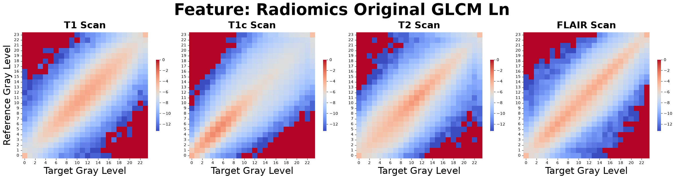
Figure: Log-normalized Gray-Level Co-occurrence Matrices (GLCM) derived from T1, T1c, T2, and FLAIR MRI sequences.

• Interpretation: The GLCM measures high-frequency, local texture. Matrices with high values clustered tightly along the diagonal indicate a highly homogeneous tumor. Values scattered far from the diagonal indicate high local contrast and chaotic texture.

• GLAM Implementation: Computed symmetrically across all 13 unique 3D directions to ensure rotational invariance.

Gray-Level Run Length Matrix (GLRLM)

Instead of looking at pairs, the GLRLM looks at continuous 1D arrays of voxels. It quantifies the number of continuous “runs” of identical gray-level voxels in a specific direction.

The matrix element \(P(i,j)\) represents the number of times a run of gray-level \(i\) occurs with a length of exactly \(j\) voxels.

\[P(i,j) = \text{Count of runs with gray-level } i \text{ and length } j\]

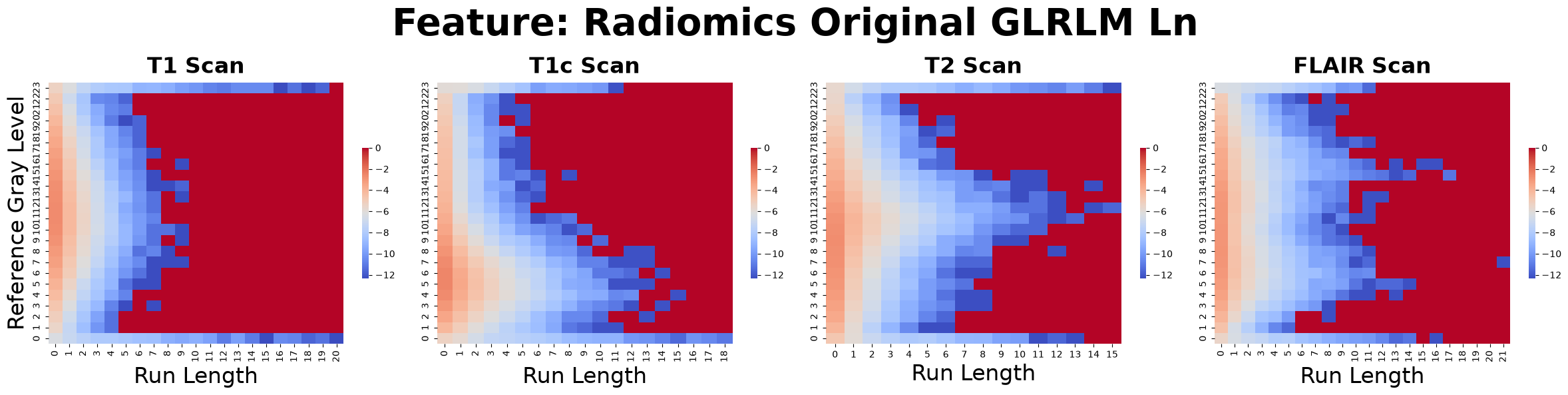
Figure: Log-normalized Gray-Level Run Length Matrices (GLRLM). The x-axis represents the Run Length in voxels.

• Interpretation: The GLRLM captures linear structures, streaks, and directional fibers. Short runs indicate fine, grainy textures, while long runs characterize coarse, smooth biological fields (like sweeping edema).

Gray-Level Size Zone Matrix (GLSZM)

The GLSZM is the 3D isotropic evolution of the GLRLM. Rather than measuring 1D linear runs, it measures the volume of fully connected 3D zones of identical gray-levels.

The matrix element \(P(i,j)\) represents the number of fully connected 3D zones of gray-level \(i\) that have a volume of exactly \(j\) voxels.

\[P(i,j) = \text{Count of 3D zones with gray-level } i \text{ and volume } j\]

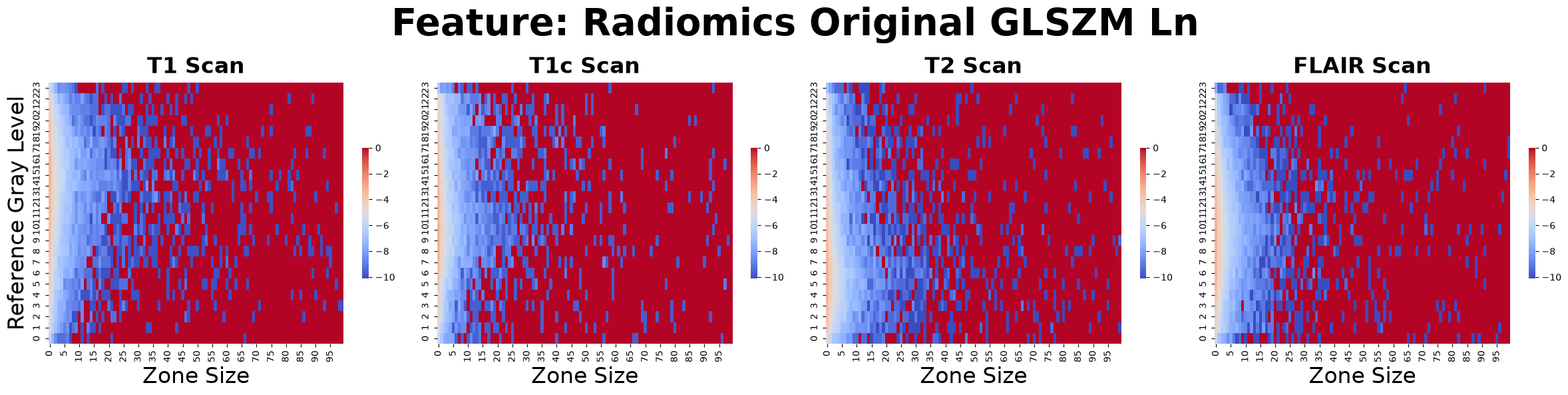
Figure: Log-normalized Gray-Level Size Zone Matrices (GLSZM). The x-axis represents the total connected volume (Zone Size) of the tissue cluster.

• Interpretation: The GLSZM is direction-independent and perfectly suited for identifying large, macroscopic tumor sub-regions. A matrix heavily weighted toward large zone sizes indicates massive, contiguous tissue architectures, such as a solid necrotic core.

Gray-Level Dependence Matrix (GLDM)

The GLDM quantifies gray-level dependencies within a specific neighborhood. A voxel is considered “dependent” on a center voxel if their gray levels are identical (or within a specified threshold).

The matrix element \(P(i,j)\) represents the number of voxels with gray-level \(i\) that have exactly \(j\) dependent voxels in their immediate 3D neighborhood.

\[P(i,j) = \text{Count of voxels of level } i \text{ with } j \text{ dependent neighbors}\]

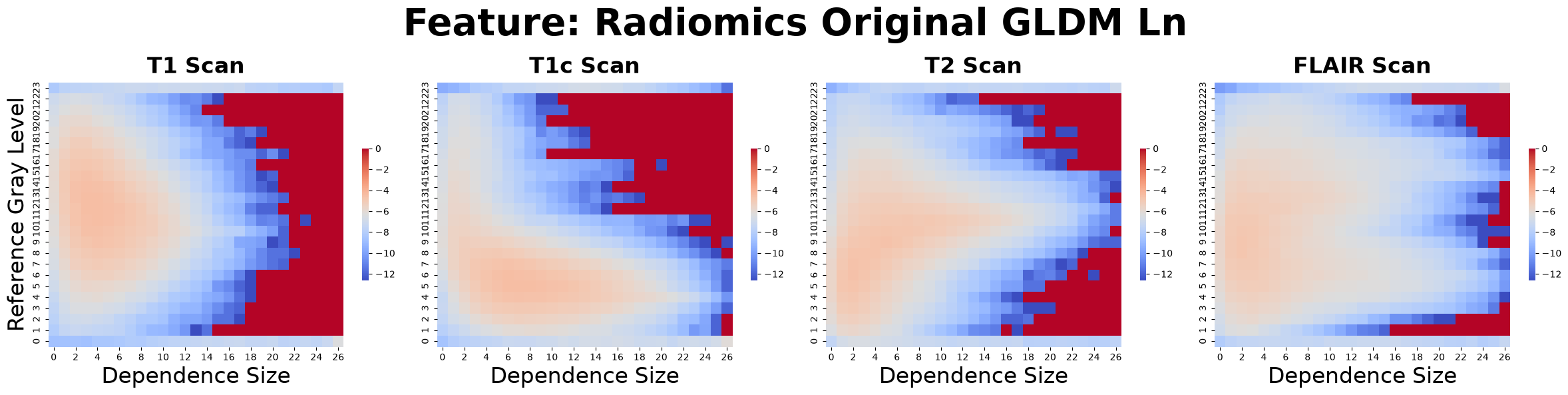
Figure: Log-normalized Gray-Level Dependence Matrices (GLDM). The x-axis represents the number of dependent neighboring voxels.

• Interpretation: GLDM measures the “coarseness” of a texture. High dependence (large \(j\) values) indicates that voxels exist in large, homogenous neighborhoods.

Neighborhood Gray-Tone Difference Matrix (NGTDM)

The NGTDM evaluates the spatial heterogeneity of an image by quantifying the difference between a voxel’s gray level and the average gray level of its immediate 3D neighborhood.

The element \(s(i)\) is calculated as the sum of absolute differences between all voxels with gray-level \(i\) and their respective neighborhood averages.

\[s(i) = \sum_{k=1}^{N_i} \left| i - \bar{A}_k \right|\]

where \(N_i\) is the number of voxels with gray level \(i\), and \(\bar{A}_k\) is the average gray level of the neighborhood surrounding the \(k\)-th voxel.

• Interpretation: The NGTDM is designed to directly capture human visual perceptions of texture. High values correspond to “busy” or high-contrast textures with rapid spatial intensity changes. Low values indicate smooth, homogeneous biological regions where voxels closely resemble their neighbors.

Log10 Transformation and Normalization

Standard radiomic matrices often exhibit an extreme dynamic range. For instance, a homogeneous background or dominant core might cause certain co-occurrences or zone sizes to reach counts in the millions, while subtle, critical tumor textures occur only a few dozen times. Left untreated, these massive numerical spikes completely overshadow the rest of the feature space.

To resolve this, logarithmic transformations (such as the \(\log_{10}\) or natural log \(\ln\) scales seen in the figures above) are regularly applied to the raw matrix counts in GLAM radiomics:

\[P_{log}(i,j) = \log_{10}(P(i,j) + 1)\]

• Visual Clarity: By compressing the dynamic range, the log transformation acts as a visual equalizer. It reveals intricate, low-frequency structural details (like rare long-runs in the GLRLM or off-diagonal interactions in the GLCM) that would otherwise be entirely invisible next to massive background peaks.

• Algorithmic Stability: Downstream machine learning models are highly sensitive to unscaled data. Log-normalization strictly prevents features with massive raw counts from dominating gradient updates or distance calculations during model training.

• Statistical Normality: The transformation converts highly skewed, heavy-tailed raw count distributions into more symmetric, Gaussian (normal) profiles, fundamentally satisfying the strict assumptions required by standard parametric statistical tests.

Dynamic Matrix Trimming in GLAM

A fundamental issue in conventional radiomics software is memory inefficiency. In a large tumor, a GLSZM might theoretically need 50,000 columns to account for the largest possible zone size, resulting in a matrix that is 99.9% empty zeroes.

GLAM natively solves this using Dynamic Matrix Trimming. During GPU extraction, GLAM precisely tracks the maximum run length or zone size actually present in the specific tumor. It then dynamically truncates the matrix columns right after the final data point. This significantly accelerates downstream feature extraction (like Entropy and Energy calculations) and dramatically reduces memory overhead without losing a single drop of mathematical precision.