Geometric Classes
Beyond statistical mechanics, the GLAM framework integrates descriptors from geometry and topology to characterize the spatial arrangement and complexity of biological textures. These metrics are organized into three primary domains:
Structural and Directional Organization
These metrics characterize how tissue components are packed and oriented within the tumor microenvironment.
Coordination Number (CN)
The Coordination Number (CN) measures the local packing or clustering of gray-levels. Adapted from atomic coordination in materials science, it represents the average number of \(\beta\)-voxels surrounding a reference \(\alpha\)-voxel within the first coordination shell:
where \(\rho_\beta\) is the mean voxel density and \(r_{min}\) is the first RDF minimum beyond the primary peak. Diagonal terms describe local self-clustering (e.g., tumor cell density), whereas off-diagonal elements quantify the degree of direct interfacing between cancerous and stromal tissue.
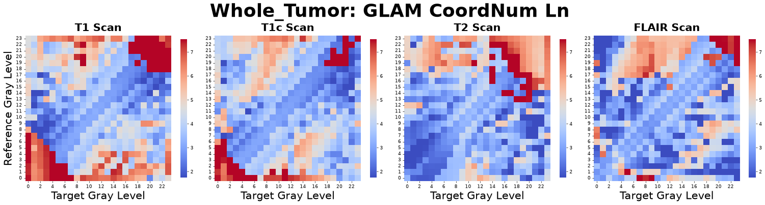
Figure: Coordination Number matrices derived from four co-registered MRI sequences: pre-contrast T1-weighted (T1), post-contrast T1-weighted (T1c), T2-weighted (T2), and Fluid-Attenuated Inversion Recovery (FLAIR).
Interpretation: This metric asks, “On average, how many immediate neighbors of type B does a central voxel of type A physically touch?”
Advantage: It provides a direct, intuitive measure of local packing density and the physical extent of the immediate contact boundary between different tissue types.
Inverse Correlation Length (Decay Rate, \(\kappa\))
The Radial Distribution Function typically exhibits an exponential decay as distance increases, reflecting the transition from short-range structural order to long-range randomness. GLAM quantifies this decay rate:
where \(\kappa\) is the Inverse Correlation Length (or Decay Rate).
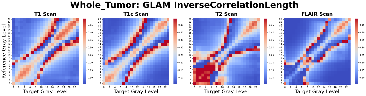
Figure: Inverse Correlation Length matrices derived from four co-registered MRI sequences: pre-contrast T1-weighted (T1), post-contrast T1-weighted (T1c), T2-weighted (T2), and Fluid-Attenuated Inversion Recovery (FLAIR).
Interpretation: A high decay rate (\(\kappa > 0\)) indicates tightly packed, highly structured local tissue domains (rapid loss of correlation). A decay rate approaching exactly \(0.0\) indicates a completely flat, random tissue distribution (a “gas-like” state) with infinite correlation length.
Advantage: By fitting the decay rate (\(\kappa\)) directly rather than the positional correlation length (\(\xi = 1/\kappa\)), the GLAM mathematical domain is safely bounded. This prevents asymptotic explosions to infinity when analyzing highly random or diffuse tissues, ensuring absolute stability for downstream machine learning algorithms.
Anisotropy Indices
GLAM captures directional organization (e.g., in aligned stromal bands) using gyration and nematic ordering tensors.
Positional Anisotropy: Uses the Relative Shape Anisotropy index, \(A_{\alpha,\beta}\), to quantify geometric elongation derived from the eigenvalues of the local gyration tensor.
Orientational Anisotropy: Calculates the Nematic Order Parameter (\(S\)), analogous to liquid crystal physics, to quantify the degree of alignment of local intensity gradients. \(S=0\) represents random orientation, while \(S=1\) indicates perfect alignment.
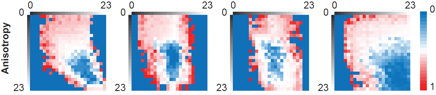
Figure: Anisotropy matrices derived from four co-registered MRI sequences: pre-contrast T1-weighted (T1), post-contrast T1-weighted (T1c), T2-weighted (T2), and Fluid-Attenuated Inversion Recovery (FLAIR).
Interpretation: This metric asks, “Are the tissue structures stretched out and aligned in a specific direction, or are they perfectly round and directionless?”
Advantage: It captures directional gradients and structural elongation, which are critical for identifying invasive fronts, aligned collagen tracks, or collective cell migration patterns.
Complexity and Topology
These measures describe the roughness, multiscale nature, and connectivity of image features.
Fractal and Multifractal Dimensions
GLAM utilizes a 3D box-counting algorithm to quantify multiscale self-similarity and complexity.
Volume Fractal Dimension (\(D_V\)): Calculated for voxels of a single gray level, indicating its space-filling capacity.
Interface Fractal Dimension (\(D_I\)): Measures the roughness and invasiveness of boundaries between two tissue types.
Multifractal Spectrum: Employs Generalized Dimensions (\(D_q\)) to characterize tissues where scaling properties vary across the region. The spectrum width (\(\Delta\alpha\)) quantifies the diversity of scaling behaviors, representing the “heterogeneous chaos” of the tissue.
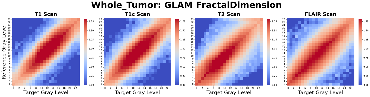
Figure: Fractal Dimension matrices derived from four co-registered MRI sequences: pre-contrast T1-weighted (T1), post-contrast T1-weighted (T1c), T2-weighted (T2), and Fluid-Attenuated Inversion Recovery (FLAIR).
Interpretation: This metric asks, “How complex, branching, and space-filling is this tissue structure across different zoom levels?”
Advantage: It captures the self-similar “roughness” of biological tissues, allowing for robust differentiation between smooth, encapsulated tumors and highly invasive, branching morphologies.
Lacunarity (\(\Lambda\))
While fractal dimension quantifies space-filling, Lacunarity measures the “gappiness” or heterogeneity of void spaces within the tissue architecture. High Lacunarity indicates large, irregular gaps, while low values suggest a uniform, homogeneous distribution.
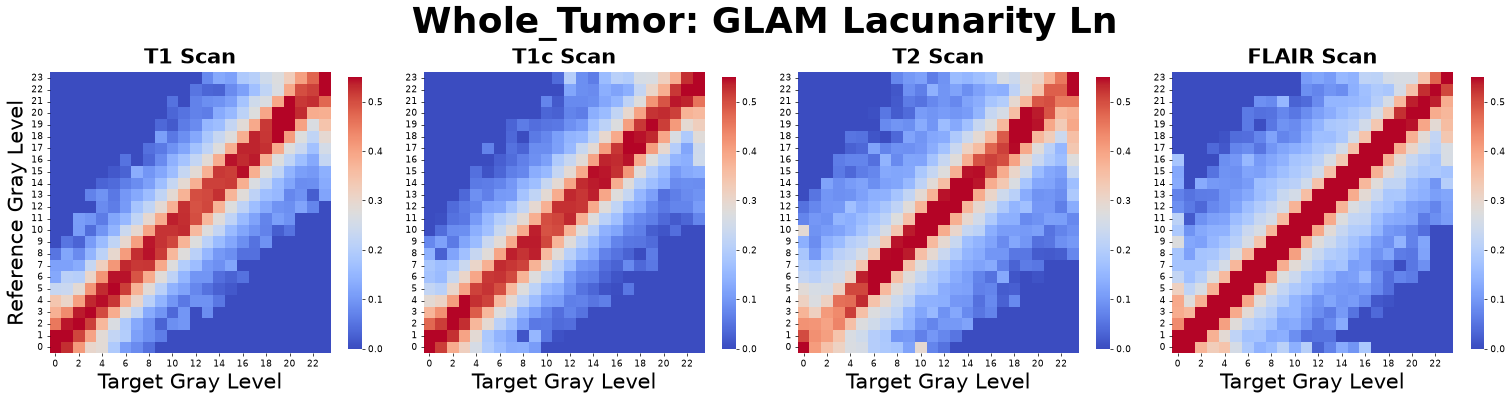
Figure: Lacunarity matrices derived from four co-registered MRI sequences: pre-contrast T1-weighted (T1), post-contrast T1-weighted (T1c), T2-weighted (T2), and Fluid-Attenuated Inversion Recovery (FLAIR).
Interpretation: This metric asks, “How complex, branching, and space-filling is this tissue structure across different zoom levels?”
Advantage: It captures the self-similar “roughness” of biological tissues, allowing for robust differentiation between smooth, encapsulated tumors and highly invasive, branching morphologies.
Topological Invariants (Betti Numbers)
GLAM uses algebraic topology to count discrete features that are invariant under continuous deformation:
Betti-0 (:math:`B_0`): Counts fragmented “islands” of a specific gray level.
Betti-1 (:math:`B_1`): Counts tunnels or loops (e.g., vascular networks).
Betti-2 (:math:`B_2`): Counts enclosed internal cavities or voids.
Euler Characteristic (:math:`chi`): A classic measure of topological complexity, where \(\chi = B_0 - B_1 + B_2\).
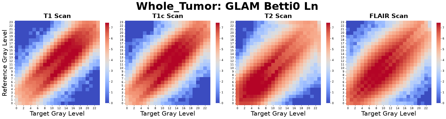
Figure: Betti0 matrices derived from four co-registered MRI sequences: pre-contrast T1-weighted (T1), post-contrast T1-weighted (T1c), T2-weighted (T2), and Fluid-Attenuated Inversion Recovery (FLAIR).
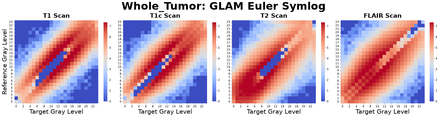
Figure: Euler Characteristic matrices derived from four co-registered MRI sequences: pre-contrast T1-weighted (T1), post-contrast T1-weighted (T1c), T2-weighted (T2), and Fluid-Attenuated Inversion Recovery (FLAIR).
Interpretation: This metric asks, “How many distinct islands, connective tunnels, and hollow voids exist within the tissue, regardless of their exact physical shape?”
Advantage: Topology is completely invariant to stretching, bending, or scaling. This makes Betti numbers incredibly robust against patient positioning differences, organ deformation, and imaging variations.
Discrete Morphology
This category extracts explicit geometric descriptors for distinct tissue clusters identified by gray-level thresholds.
Sphericity and Solidity: Measure the compactness and “ruggedness” of individual gray-level isosurfaces.
Interface Area: Quantifies the total surface of direct contact between two distinct tissue types, representing the extent of physical infiltration.
Centroid Distance: Measures the Euclidean distance between the centers of mass of different tissue components.
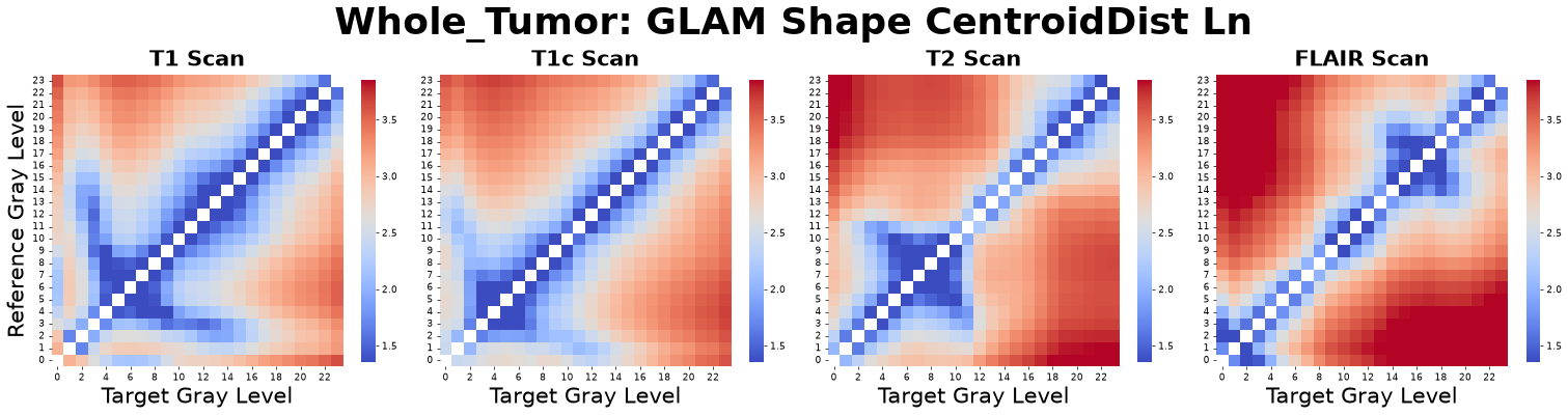
Figure: Centroid Distance matrices derived from four co-registered MRI sequences: pre-contrast T1-weighted (T1), post-contrast T1-weighted (T1c), T2-weighted (T2), and Fluid-Attenuated Inversion Recovery (FLAIR).
Interpretation: This metric asks, “What are the tangible physical dimensions, roundness, and contact areas of these specific tissue clumps?”
Advantage: It provides highly tangible, classic geometric descriptors that correlate directly with standard visual pathological assessments.
Percolation Metrics
Percolation theory evaluates the connectivity of voxel clusters to determine how local tissue states connect to form macroscopic, spanning networks. It bridges the gap between local discrete morphology and global tissue architecture by quantifying whether a specific tissue type forms a continuous network or exists as isolated fragments. GLAM quantifies this using three primary matrices:
Maximum Cluster Size (\(S_{max}\)): The absolute voxel count of the largest connected cluster of a specific gray level. It represents the raw biological burden of the largest continuous region (e.g., the absolute volume of the largest contiguous necrotic core).
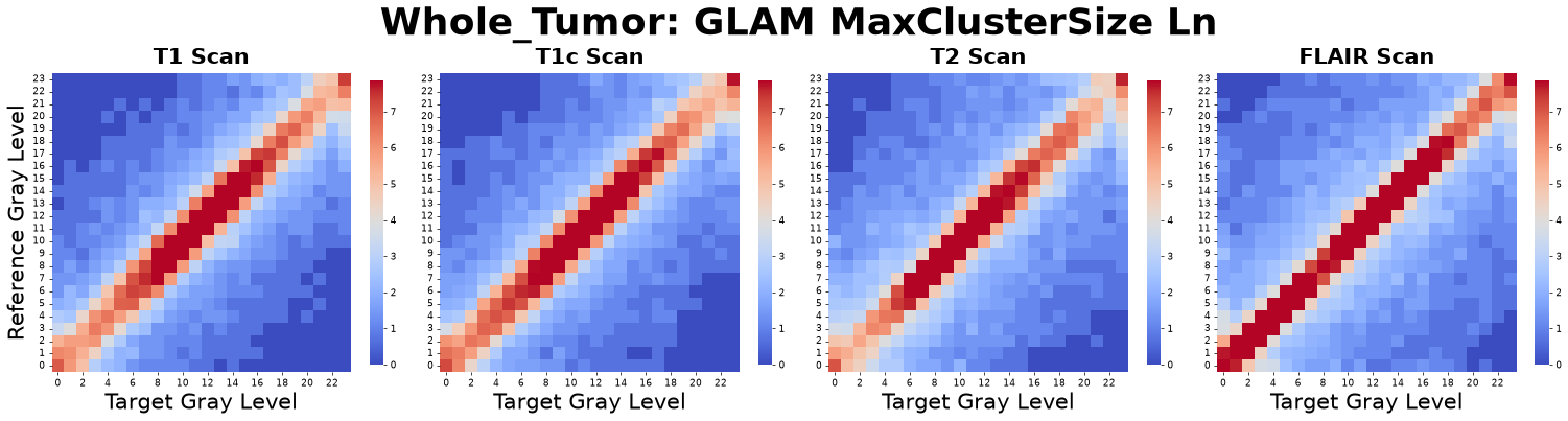
Figure: Maximum Cluster Size matrices derived from four co-registered MRI sequences: pre-contrast T1-weighted (T1), post-contrast T1-weighted (T1c), T2-weighted (T2), and Fluid-Attenuated Inversion Recovery (FLAIR).
Cluster Number Density (\(n_c\)): The total number of isolated clusters normalized by the total ROI volume (\(N_{clusters} / V_{ROI}\)). It quantifies the degree of macroscopic fragmentation.
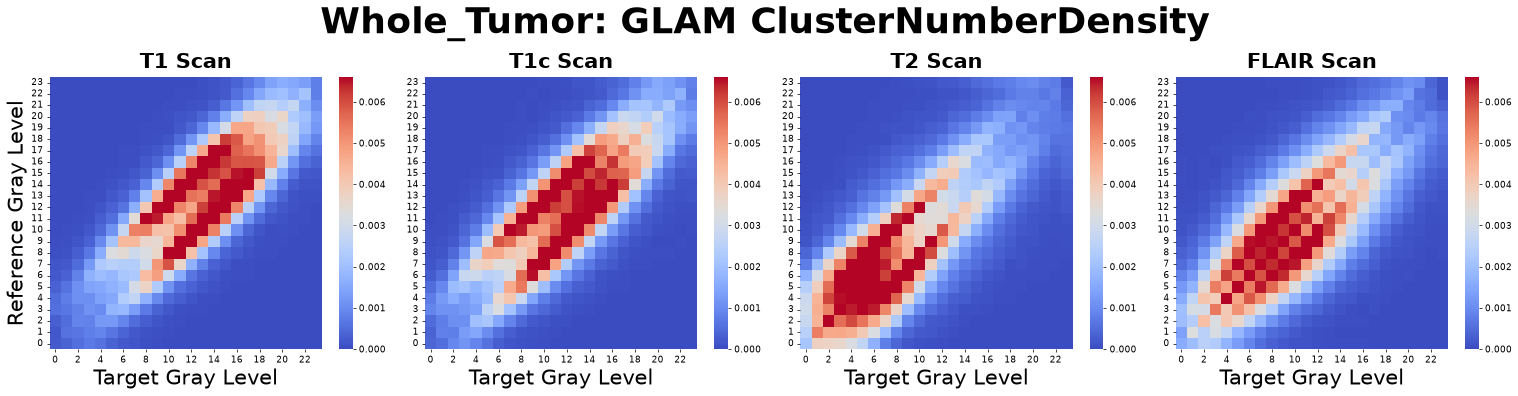
Figure: Cluster Number Density matrices derived from four co-registered MRI sequences: pre-contrast T1-weighted (T1), post-contrast T1-weighted (T1c), T2-weighted (T2), and Fluid-Attenuated Inversion Recovery (FLAIR).
Percolation Strength ( \(P\) ): The probability that any active site belongs to the largest cluster, defined as \(P = S_{max} / N_{active}\). This provides a volume-independent, static surrogate for the percolation threshold, allowing robust texture comparisons between tumors of vastly different sizes.
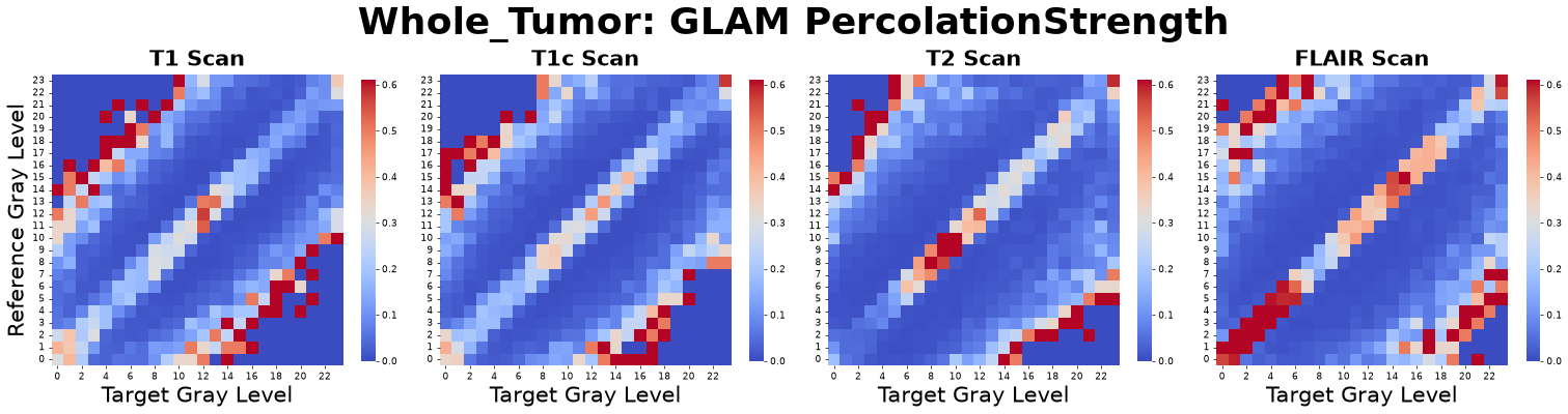
Figure: Percolation Strength matrices derived from four co-registered MRI sequences: pre-contrast T1-weighted (T1), post-contrast T1-weighted (T1c), T2-weighted (T2), and Fluid-Attenuated Inversion Recovery (FLAIR).
Interpretation: This metric asks, “Is this specific tissue type organized into one massive, connected network that spans the tumor, or is it shattered into tiny, disconnected islands?”
Advantage: By providing both the absolute biological burden (\(S_{max}\)) and the normalized, scale-invariant network connectivity (\(P\)), percolation metrics preserve critical volumetric context for clinical staging while enabling mathematically pure, volume-independent texture comparisons across heterogeneous patient cohorts.
Granulometry (Pattern Spectrum)
Granulometry, or morphological sieving, calculates the physical thickness distribution of distinct tissue states. While percolation evaluates network connectivity, granulometry filters the region using spherical structuring elements of increasing radii to extract a Pattern Spectrum \(P(r)\).
Granulometry Mean: Represents the average localized thickness of a gray-level cluster or interface.
Granulometry Variance & Entropy: Quantifies the structural heterogeneity (e.g., measuring “sponginess” by detecting a highly unpredictable mix of thin offshoots and thick bulk nodes).
Granulometry Skewness & Kurtosis: Identifies morphological imbalance. A positive skew indicates a cluster dominated by thin, fragmented bridges with only rare, exceptionally thick regions.
Interpretation: This metric asks, “What is the physical thickness profile of this specific tissue type, and is it built like a solid, uniform mass or a spongy, highly variable structure?”
Advantage: While standard size metrics (like GLSZM) measure total cluster volume regardless of shape, granulometry isolates the true physical width and granularity. This perfectly distinguishes between a solid tumor core and a diffuse, spindly network of the exact same volume—a critical distinction in delta radiomics when monitoring tissue breakdown or cavitation during therapy.
Topological Excess Features (Excess Matrices)
Excess Matrices (\(\Delta M\)) quantify the degree to which a specific topological property—such as fragmentation, porosity, or cavitation—deviates from a purely random spatial distribution. In the GLAM pipeline, these matrices are generated for all primary topological metrics: Betti-0 (fragments), Betti-1 (tunnels/loops), Betti-2 (voids), and the Euler Characteristic.
To calculate an Excess Matrix, the pipeline first computes the structured topological state of the tumor. It then generates a randomized “null model” by randomly shuffling the spatial positions of all voxels within the region of interest (ROI). This preserves the exact density of each gray level but destroys all spatial correlations. The topology of this null model is calculated, and the excess is defined as the arithmetic difference between the structured and random states:
Where:
\(M\) represents the target topological metric (e.g., \(\beta_0\), \(\beta_1\), \(\beta_2\), or \(\chi\)).
\(i, j\) represent the interacting gray levels. If \(i=j\), it represents the volumetric topology of a single tissue; if \(i \neq j\), it represents the topology of the interface between two tissues.
\(M(i, j)_{\text{structured}}\) is the measured topological feature in the actual tumor image.
\(M(i, j)_{\text{random}}\) is the expected topological feature if the tissue voxels were mixed perfectly at random.
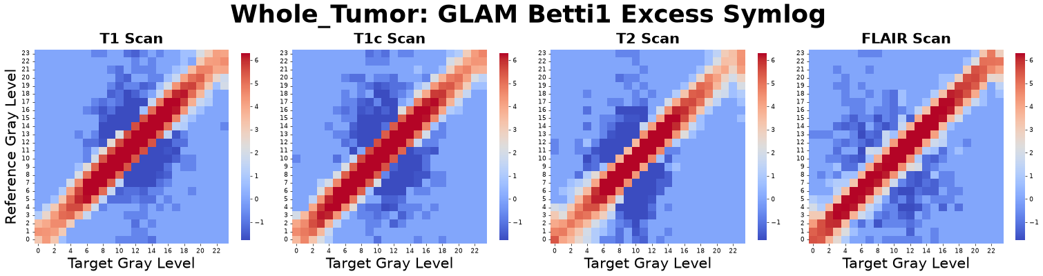
Figure: Betti-1 Excess matrices (Symlog) derived from four co-registered MRI sequences: pre-contrast T1-weighted (T1), post-contrast T1-weighted (T1c), T2-weighted (T2), and Fluid-Attenuated Inversion Recovery (FLAIR).
General Interpretation:
Negative Excess (\(\Delta M < 0\)): The spatial architecture is highly ordered to suppress this specific topological feature compared to random noise.
Positive Excess (\(\Delta M > 0\)): The biological architecture actively amplifies this topological feature beyond what statistical chance would produce.
Zero Excess (\(\Delta M \approx 0\)): The topological arrangement of the tissue is indistinguishable from a purely random mixture.
Metric-Specific Biological Context:
Betti-0 Excess (Fragmentation): Negative excess indicates strong spatial aggregation and cohesion (large, continuous tumor masses). Positive excess indicates severe tissue shattering or diffuse biological scattering.
Betti-1 Excess (Porosity/Loops): Negative excess implies a solid, non-porous structure. Positive excess suggests a highly interconnected, spongy, or web-like tissue architecture (often seen in complex vascular/stromal networks).
Betti-2 Excess (Cavitation/Voids): Negative excess indicates dense tissue with few internal pockets. Positive excess points to significant internal cavitation, such as isolated necrotic cores, fluid pockets, or cysts.